Google Spreadsheet Differentiating 1 and 11 in find formula

Question:

( by Dave Viola )

In a spreadsheet, I'm trying to extract numbers (that represent grade levels) and text from a single cell (filled by a checkbox item on a form), to spread them across rows, so that users can sort the sheet.

The data from the form is in a comma-separated list, so:  K,1,2,6,7,8 for example.

Some of the form entries have multiple grade levels, some of the entries have a single grade level, and some have ranges that skip grade levels in between; so the easiest way I thought of to do this was to follow the initial entry with 13 columns (K, 1, 2, 3, 4, 5, 6, 7, 8, 9, 10, 11, 12), and then just have each column fill if the corresponding row is intended for that grade level -- therefore, all the 7th grade teachers could search for 7th grade items only, etc.

Here's the formula I used in the columns to the right of the column which has all of the data (in this case, H@):  =IFERROR(IF(Find("01",H2)>0,1),"")

I could not figure out a way to separate the entries for grade 1 from the entries from grade 11, unless all the grades were entered as double digit (01, 02, etc.), which is ungainly.

Is there a better way to do this?

Using Chrome, and OSX 10.8.4

======

Thanks for the suggestions -- but wouldn't those initial commands only find 1 or 11 if they were embedded inside commas?  If a respondent only chooses "1" in the Google Form (they're entering data from there), then the cell only has 1 in it, no commas, and no spaces.

I thought about the split command, but since it doesn't sort the data, it wouldn't always put the same digits in the same columns -- (so, a cell containing "1,2,3,4" would be split so the 4 is in the 4th column to the right, but a cell containing "4,5,6" would be split so the 4 ends up in the first cell to the right of the initial cell.)

a) The spreadsheet is here:

b) The source of the data for the formula is on the sheet 'Master,' in column H; I'd like the results to be spread across columns M-Y.

So, the expected result would be to have the entry in column H, like "K,1,2,5,6,7" split into the appropriate rows in M-Y, so the K would end up in the "K" column (column M), the 1 in the "1" column.  The difficulty for me is in writing a formula that would correctly extract "1" only when 1 was entered as a single digit  -- so an entry of "11, 12" would not also populate the "1" and "2" columns (columns N and O).  

The clumsy solution I've found is to restrict the data entry options on the Google Form to "01," "02" etc., but that's slightly ungainly, because teachers tend not to think of grades that way.

Solution:

Have a look at the following screenshot:

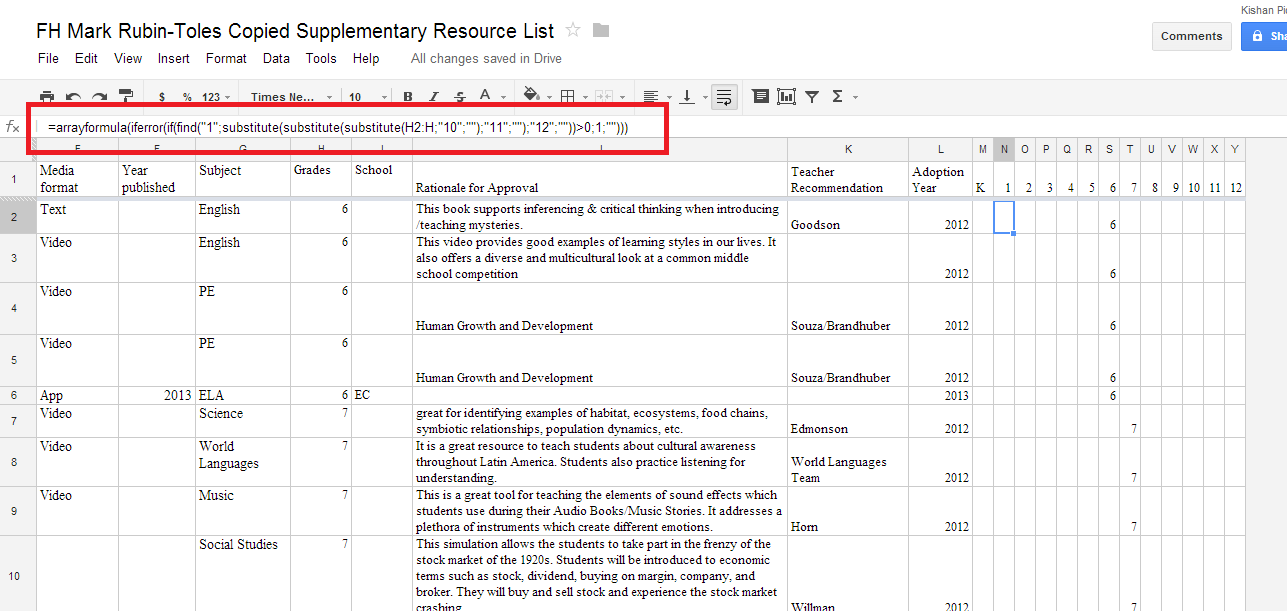
Now, instead of filling formula in each cell, you can use arrayformula to auto compute entire range.

I have inserted the following formula in Cell M2:
=arrayformula(iferror(if(find("K";H2:H)>0;"K";"")))

I have inserted the following formula in Cell N2:
=arrayformula(iferror(if(find("1";substitute(substitute(substitute(H2:H;"10";"");"11";"");"12";""))>0;1;"")))

the above formula will substitute 10,11,12 with "" (that is blank) and the it will find 1 in the remaining string. Still if it finds 1 then it will return 1 or else blank.

I have inserted the following formula in Cell O2:

=arrayformula(iferror(if(find("2";substitute(H2:H;"12";""))>0;2;"")))

I have inserted the following formula in Cell P2:
=arrayformula(iferror(if(find("3";H2:H)>0;3;"")))

I have inserted the following formula in Cell Q2:
=arrayformula(iferror(if(find("4";H2:H)>0;4;"")))

And similarly you can fill the remaining formulas...

I hope the above solution will help you, and if you need more help then please do comment below on this blog itself, I will try to help you out.

I also take up private and confidential projects:

http://igoogledrive.blogspot.com/p/paid-projects.html

If this blog post was helpful to you, and if you think you want to help me too and make my this blog survive then please donate here: http://igoogledrive.blogspot.com/2012/09/donate.html 

Thanks,

Kishan.

iGoogleDrive